name: title class: middle, center, dark <center> <embed src="images/title.svg" type="image/svg+xml" height="100px" align="center" style="border: 0px solid lightgray;"/> </center> --- class: light, center, middle, clear # Chance does things --- class: light # Big ideas for this course 1. Psychology interpets patterns in data to draw conclusions about psychological processes -- 2. Chance can produce "patterns" in data -- 3. **Problem**: How can we know if the pattern is real, or simply a random accident produced by chance --- class: light # Solutions 1. Need to understand what chance is -- 2. Need to find out what chance can actually do in a particular situation -- 3. Create tools to help us determine whether chance was likely or unlikely to produce patterns in the data --- class: light # Issues for this class 1. **Probability Basics** 2. **Distributions** 3. **Sampling from distributions** --- class: light, center, middle, clear # Probability Basics --- class: light # What is a probability? - A number bounded between 0 and 1 - Describes the "chances" or "likelihood" of an event --- class: light # Proportions and Percentages - Percentage (%) : A ratio between event frequency, and total frequency, expressed in units of 100. - Proportion : a decimal version (range between 0-1) `\(100\% = \frac{100}{100} = 1 = 1*100 = 100\%\)` `\(50\% = \frac{50}{100} = .5 = .5*100 = 50\%\)` `\(\frac{2}{4} = .5 = .5*100 = 50\%\)` --- class: light # Two probability statements - A coin has a 50% chance of landing heads - p(heads) = .5 -- - There is a 10% chance of rain tomorrow - p(rain tomorrow) = .1 --- class: light # Frequentist vs. Bayesian Probability is defined differently depending on philosophical tradition. 1. Frequentist: The long-run chances (odds) of an event occurring 2. Bayesian: Degree of belief --- class: light # A fair coin A fair coin has a 50% chance of landing heads or tails - Frequentist: If you flip this coin an infinity of times, **in the long run** half of the outcome will be heads, and half will be tails - Bayesian: I am uncertain about the outcome, I can't predict what it will be. --- class: light # 10% chance of rain tomorrow 10% chance of rain tomorrow refers to a single event that hasn't yet occurred - Frequentist: I don't know what to say. Tomorrow it will rain or not rain, so there will be a 0% or 100% chance of rain, we'll find out after tomorrow happens - Bayesian: It is unlikely to rain tomorrow, I won't bring an umbrella. --- class: light, center, middle, clear # 50% chance --- class: light # Coin flipping I made Python flip a fair coin 100 times: ``` ## [,1] [,2] [,3] [,4] [,5] [,6] [,7] [,8] [,9] [,10] ## [1,] "H" "H" "T" "T" "H" "H" "H" "T" "H" "T" ## [2,] "T" "H" "T" "H" "H" "H" "H" "H" "T" "H" ## [3,] "H" "H" "H" "T" "T" "T" "H" "T" "H" "T" ## [4,] "T" "T" "H" "T" "H" "H" "T" "T" "H" "T" ## [5,] "H" "T" "T" "H" "T" "T" "H" "H" "T" "T" ## [6,] "H" "H" "H" "T" "T" "T" "T" "H" "T" "T" ## [7,] "H" "H" "H" "T" "T" "T" "H" "T" "T" "H" ## [8,] "T" "T" "H" "T" "H" "H" "H" "T" "H" "H" ## [9,] "T" "T" "T" "T" "T" "H" "H" "H" "T" "H" ## [10,] "T" "H" "H" "T" "T" "H" "T" "T" "H" "T" ``` --- class: light # Flipping a coin 100 times 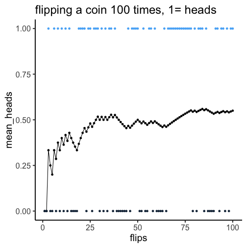<!-- --> --- class: light # Four simulations <!-- --> --- class: light # Flipping a coin 10000 times <!-- --> --- class: light # coin flipping summary 1. 50% heads/tails means that **over the long run**, you should get half heads and half tails 2. When sample size (number of flips) is small, you can "randomly" get more or less than 50% heads 3. Chance is lumpy --- class: light # Discrete probability distributions 1. Defines the probability of each item in a set. 2. All probabilities must add up to 1 --- class: light # Coin flipping distribution <!-- --> --- class: light, center, middle, clear # What can the coin flipping distribution do? --- class: light # 10 sets of 10 flips <!-- --> --- class: light # flipping a coin 10 times 1. We expect to get 5 heads and 5 tails on average 2. But, we often do not get exactly 5 heads and 5 tails 3. Randomly sampling from the distribution can produce a variety of answers --- class: light # simulating 10 flips many times Steps: 1. Flip a coin 10 times 2. count the number of heads, save the number 3. Repeat above 1,000 times or more 4. plot the histogram of number of heads --- class: light # Distribution of heads (10 flips) 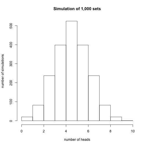<!-- --> --- class: light # Summary of simulation 1. Chance produces a range of outcomes (number of heads out of 10) 2. Chance most frequently produces 5 heads and 5 tails 3. Chance produces more extreme outcomes with increasingly less frequency (lower probability) 4. E.g., chance is very unlikely to produce 9 out of 10 heads --- class: light # flipping a coin 100 times What if we simulated flipping a coin 100 times, what would the range of outcomes be? --- class: light # flipping a coin 100 times 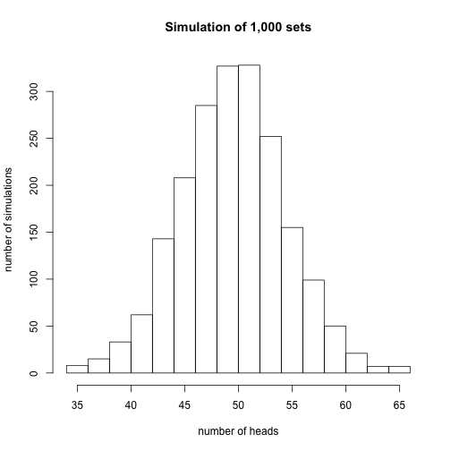<!-- --> --- class: light, center, middle, clear # Distributions --- class: light # Distributions 1. A tool to define the chances of getting particular numbers 2. Distributions have shapes 3. Higher values indicate higher chance of getting a value --- class: light # Distributions have shapes <img src="figs-crump/distribution/d1.png" width="80%" /> --- class: light # Area under the curve <img src="figs-crump/distribution/d2.png" width="80%" /> --- class: light # Interpreting distributions <img src="figs-crump/distribution/d3.png" width="80%" /> --- class: light # Point Estimates <img src="figs-crump/distribution/d4.png" width="80%" /> --- class: light # Probability ranges <img src="figs-crump/distribution/d5.png" width="80%" /> --- class: light # Uniform Distribution Definition: 1. All numbers in a particular range have an equal (uniform) chance of occuring --- class: light # Uniform Distribution <!-- --> --- class: light # Sampling from a uniform Python let's you sample numbers from a uniform distribution ``` np.random.uniform(0,1,25) ``` ``` array([0.06567211, 0.83317117, 0.77310506]) ``` ``` np.random.uniform(0,10,3) ``` ``` array([3.23770171, 3.47811007, 7.11685081]) ``` --- class: light # looking at samples <!-- --> --- class: light # Random samples are not all the same <img src="figs-crump/distribution/5manysamples-1.png" width="90%" /> --- class: light # Samples estimate the distribution 1. Samples are sets of numbers taken from a distribution -- 2. **Samples become more like the distribution they came from, as sample size (N) increases** --- class: light # Uniform: N=100 <img src="figs-crump/distribution/5unifsamp100-1.png" width="80%" /> --- class: light # Uniform: N=1,000 <img src="figs-crump/distribution/5unifsamp1000-1.png" width="80%" /> --- class: light # Uniform: N=100,000 <img src="figs-crump/distribution/5sampunifALOT-1.png" width="80%" /> --- class: light, center, middle, clear # Some questions --- class: light # Samples and distributions How do samples relate to distributions? -- - Samples come from distributions -- - Samples approximate the distribution they came from as sample-size increases --- class: light # Is my sample likely? Let's say you take a sample of numbers from a distribution. 1. Is your sample representative of the population? 2. Was your sample likely (you would usually get a sample like this), or unlikely (you got a weird sample, usually you would not get a sample like this) --- class: light # Simulation and sampling How can we know if a sample we obtained is "normal", or "weird"? -- - We can find out by simulating the process of sampling. - We sample some numbers, measure the sample, then repeat - We can now look at how our measurement of the sample behaves --- class: light # Animation of sample mean <!-- --> --- class: light # What to notice - The histogram shows that each sample is different - But, the mean of each sample is always around 5.5 - We have measured a property of the sample (the mean), each time. --- class: light # Something Curious <img src="figs-crump/distribution/4unifmany-1.png" width="592" /> --- class: light, center, middle, clear # Make sure you understand sampling distributions --- class: light, center, middle, clear # Make sure you understand this next graph --- class: light, center, middle, clear <img src="figs-crump/distribution/pop_samp.png" width="545" /> --- class: light # Big ideas for this course 1. Psychology interpets patterns in data to draw conclusions about psychological processes -- 2. Chance can produce "patterns" in data -- 3. **Problem**: How can we know if the pattern is real, or simply a random accident produced by chance --- class: light # Issues for this class 1. **Sampling distributions** 2. **Normal distributions and central limit theorem** 3. **Estimation** --- class: light, center, middle, clear # Samples and populations --- class: light # Samples and populations - Population: A defined set of things - Sample: a subset of the population --- class: light # Random Sampling - A process for generating a sample (taking things from a population) -- - Random samples ensure that each value in a sample is drawn **independently** from other values -- - all values in the population have a chance of being in the sample --- class: light # Example: Sampling heights of people Let's say we wanted to know something about how tall people are. We can't measure the entire population (it's too big). So we take a sample. -- What would happen if: 1. We only measured really tall people (biased sample) -- 2. We randomly measured a bunch of people? --- class: light # Population statistics Populations have statistics. For example, The population of all people has: 1. A distributions of heights 2. The distribution has a mean (mean height of all people) 3. The distribution has a standard deviation --- class: light # The population problem In the real world, we usually do not have all of the data for the entire population. So, we never actually know: 1. The population distribution 2. The population mean 3. The population standard deviation, etc. --- class: light # The sampling solution Unknown: The population Solution: Take a sample of the population 1. Samples will tend to look the population they came from, especially when sample-size (N) is large. 2. We can use the sample to **estimate** the population. --- class: light # The sampling problem We take samples, and use them to estimate things. This works well when we have large, representative samples. But, how do we know if the sample we obtained is "normal", or happens to be "weird"? Solution: We need to learn how the process of sampling works. We can use R to simulate the process of sampling. Then we can see how samples behave. --- class: light # Samples become populations - As sample-size increases, the sample becomes more like the population. - As sample N approaches the population N, the sample becomes the population. --- class: light # Law of large numbers - As sample-size increases, properties of the sample become more like properties of the population Example: - As sample-size increases, the mean of the sample becomes more like the mean of the population --- class: light # Simulation: Population mean=100 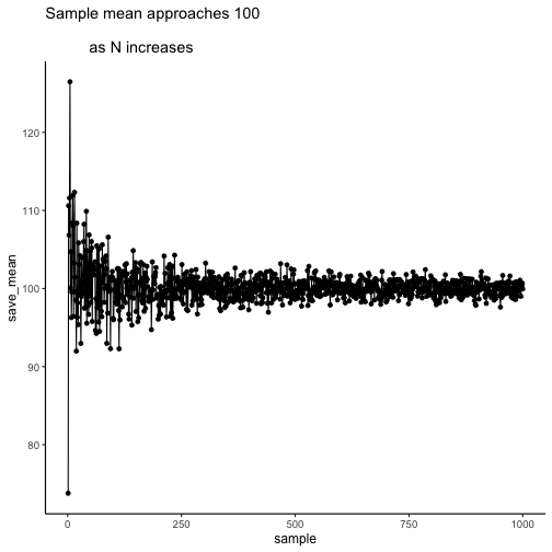<!-- --> --- class: light # The sampling problem We take samples, and use them to estimate things. This works well when we have large, representative samples. **But, how do we know if the sample we obtained is "normal", or happens to be "weird"?** Solution: **Sampling Distributions** --- class: light, center, middle, clear # Sampling distributions --- class: light # What are sampling distributions? - Definition: The distribution of a sample statistic - Example: - Many samples are drawn from the same distribution - A statistic (e.g., mean, standard deviation) is computed for each sample, and saved - The sampling distribution is the distribution of the measured statistic for each sample - Sampling distributions can be simulated in R --- class: light # Begin with a distribution <!-- --> --- class: light # Take many samples Save a sample statistic (e.g., mean) for each sample <!-- --> --- class: light # Plot distribution of sample statistic <img src="figs-crump/distribution/4unifmany-1.png" width="592" /> --- class: light # Sampling distribution is bell-shaped Notice that the sampling distribution of the mean is bell-shaped, also called a **Normal Distribution**. <img src="figs-crump/distribution/4unifmany-1.png" width="50%" /> --- class: light # Sampling distributions for anything A sampling distribution can be found for any sample statistic. 1. Choose a statistic to measure (e.g., mean, median, variance, standard deviations, max, min, etc.) 2. Measure statistics for each sample 3. Plot the sampling distribution --- class: light # A few sampling distributions <img src="figs-crump/distribution/4samplestats-1.png" width="592" /> --- class: light # Use for sampling distributions? Question: What does a sampling distribution tell us? Answer: - The distribution of values a sample statistic can take, for a sample of a particular size In other words, - Gives us information about range and probability of obtaining particular sample statistics --- class: light # Sampling distribution of the mean <img src="figs-crump/distribution/4unifmany-1.png" width="592" /> --- class: light # Standard error of the mean (SEM) - Definition: the standard deviation of the sampling distribution of the sample means Formulas: Can be computed directly for samples of any size if you know the standard deviation of the population distribution. `\(\text{SEM}=\frac{\text{standard deviation}}{\sqrt{N}}\)` `\(\text{SEM}=\frac{\sigma}{\sqrt{N}}\)` `\(\sigma\)` = population standard deviation --- class: light # SEM What does the SEM (standard error of the mean) tell you. - Let's say your sample mean was 5, and the SEM was 2. - The SEM is the standard deviation of the sampling distribution of the sample mean - Now you know that your sample mean is 5, but as an estimate of the population mean, that number varies a little bit. SEM tells you how much in standard deviation units. --- class: light # Central limit theorem With enough samples, sampling distributions are approximately **normal distributions** - Sampling distributions have the same shape as a normal distribution, even when the distribution that the sample came from does not have a normal shape. --- class: light, center, middle, clear # Normal Distributions --- class: light # Normal distributions are bell-shaped <img src="figs-crump/distribution/standardNormal-eps-converted-to.png" width="80%" /> --- class: light # Normal distribution formula <img src="figs-crump/distribution/Normal_formula.png" width="715" /> --- class: light # Normal distribution parameters Normal distributions have two important parameters that change their shape: 1. The mean (where the peak of the distribution is centered) 2. The standard deviation (how spread out the distribution is) --- class: light # Normal: Changing the mean <!-- --> --- class: light # Normal: Changing standard deviation <!-- --> --- class: light # rnorm() R has a function for generating numbers from a normal distribution. - n = number of samples - mean = mean of distribution - sd = standard deviation of distribution ```r rnorm(n=100, mean = 50, sd = 25) ``` --- class: light # plotting a sample from a normal ```r hist(rnorm(n=100, mean=50, sd=25)) ``` <img src="4b_Sampling_files/figure-html/unnamed-chunk-14-1.png" width="60%" /> --- class: light # increasing N ```r hist(rnorm(n=1000, mean=50, sd=25)) ``` <img src="4b_Sampling_files/figure-html/unnamed-chunk-15-1.png" width="60%" /> --- class: light # Animating the central limit theorem <!-- --> --- class: light # Normal & central limit <img src="figs-crump/distribution/4sampledistmeannorm-1.png" width="592" /> --- class: light # Uniform & central limit <img src="figs-crump/distribution/4samplemeanunif-1.png" width="592" /> --- class: light # exponential & Central limit <img src="figs-crump/distribution/4samplemeanExp-1.png" width="592" /> --- class: light # Importance of central limit theorem 1. We see that our sample statistics are distributed normally 2. We can use our knowledge of normal distributions to help us make inferences about our samples. Question: A. What do we need to know about the normal distribution to make use of it? --- class: light # Normal distributions and probability <img src="figs-crump/distribution/4normalSDspercents-1.png" width="592" /> --- class: light # Normal distributions and probability <img src="figs-crump/distribution/4normalSDspercentsB-1.png" width="592" /> --- class: light # pnorm() Use the `pnorm()` function to determine the proportion of numbers up to a particular value q = quantile What proportion of values are smaller than 0, for a normal distribution with mean =0, and sd= 1? ```r pnorm(q=0, mean= 0, sd =1) ``` ``` ## [1] 0.5 ``` --- class: light # pnorm() continued What proportion of values are between 0 and 1, for a normal distribution with mean =0, and sd =1? ```r lower_value <- pnorm(q=0, mean= 0, sd =1) higher_value <- pnorm(q=1,mean=0, sd=1) higher_value-lower_value ``` ``` ## [1] 0.3413447 ``` --- class: light, center, middle, clear # Estimation --- class: light # Goals of estimation - Use statistics of samples to estimate the statistics of the population (parent distribution) they came from - Use statistics of samples to estimate "error" in the sample --- class: light # Biased vs. unbiased estimators Biased estimators: Sample statistics that are give systematically wrong estimates of a population parameter Unbiased estimators: Sample statistics that are not biased estimates of a population parameter --- class: light # Sample means are unbiased - The mean of a sample is an unbiased estimator of the population mean --- class: light # Sample demonstration <!-- --> --- class: light # Standard deviation is biased - The standard deviation formula (dividing by N) is a **biased** when applied to a sample, is a biased estimator of the population standard deviation. Formula for Population Standard Deviation `\(\text{Standard Deviation} = \sqrt{\frac{\sum{(x_{i}-\bar{X})^2}}{N}}\)` --- class: light # Sample demonstration <!-- --> --- class: light # Sample Standard Deviation - If we divide by N-1, which is the formula for a sample standard deviation, we get an **unbiased** estimate of the population standard deviation Formula for **Sample Standard Deviation** `\(\text{Standard Deviation} = \sqrt{\frac{\sum{(x_{i}-\bar{X})^2}}{N-1}}\)` --- class: light # Sample demonstration <!-- --> --- class: light, center, middle, clear <img src="figs-crump/distribution/pop_samp.png" width="645" /> --- class: light # sd() and SEM in R `sd()` computes the standard deviation using N-1 ```r x <- c(4,6,5,7,8) sd(x) ``` ``` ## [1] 1.581139 ``` SEM is estimate of standard deviation divided by square root of N ```r sd(x)/sqrt(length(x)) ``` ``` ## [1] 0.7071068 ``` --- class: light # Questions for yourself 1. What is the difference between a population mean and sample mean? 2. What is the difference between a population standard deviation and sample standard deviation? 3. There are two standard deviation formulas for a sample, one divides by N, and the other divided by N-1. What is the difference between the two? --- class: light # More questions 1. What is a sampling distribution, how is it different from a single sample? 2. What is the sampling distribution of the sample means? 3. What is the standard error of the mean (SEM), and how does it relate to the sampling distribution of the sample means? --- class: light # Even more questions 1. What is the difference between the standard error of the mean, and the estimated standard error of the mean? --- class: light Thanks to Matt Crump (Brooklyn College) for some of the slides.